Guitar Pickup Equivalent Circuits
Posted on Sun 18 June 2023 in Articles
Summary~
An equivalent circuit of a guitar's pickups, tone/volume controls and cable is useful when designing input stages for effects pedals or amplifiers. It makes simulations or calculations of how input networks modify the spectrum of the guitar's output more realistic. This article covers some background on the topic and then goes into a technique for measuring the output impedance of a guitar and how to deduce the values of an equivalent circuit from the measurement.
The actual values that I found for the equivalent circuit of a Stratocaster are given in the Conclusion at the end of this page.
Contents~
Introduction~
A magnetic guitar pickup is essentially a coil of wire that is used as an inductive sensor. A fairly standard equivalent circuit for a non-ideal inductor adds a series resistor representing the resistance of the windings and a parallel capacitor representing the capacitance between the windings. Combinations of pickups, pickup selector switches, tone controls and volume controls all contribute to the output impedance of a guitar but for these the connections and component values are almost always available so the "equivalent circuit" is simply the actual circuit.
The schematic below shows a fairly complete equivalent circuit for a single pickup with tone and volume controls which describes for example the bridge pickup of a Stratocaster. The format of the circuit was inspired by the introduction of Rod Elliott's article entitled 'Zero Capacitance' Guitar Lead.
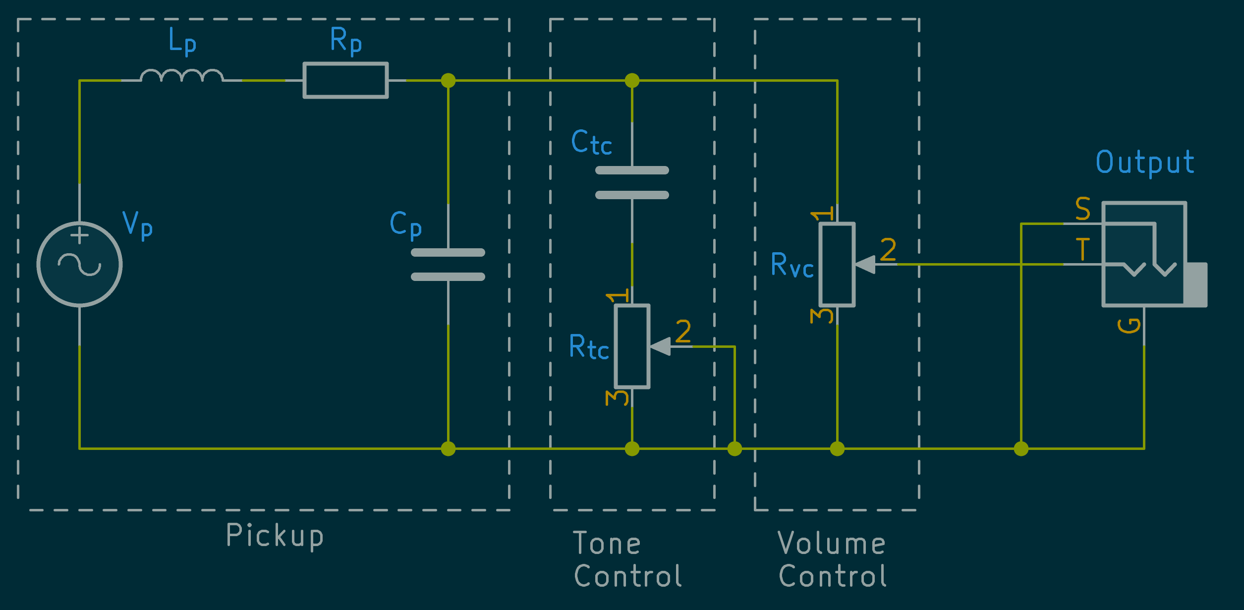
| Symbol | Meaning |
|---|---|
| Vp | Pickup signal voltage i.e. the voltage induced in the pickup by the moving string |
| Lp | Pickup winding inductance |
| Rp | Pickup resistance |
| Cp | Pickup winding capacitance |
| Ctc | Tone control capacitance |
| Rtc | Tone control potentiometer resistance |
| Rtc | Volume control potentiometer resistance |
There are a lot of potential combinations of control and switch settings, so for brevity this article will just consider a single pickup with no tone control and set to maximum volume.
Guitar cables typically have equivalent shunt capacitances of at least 50 pF/m (see here for examples) so for any cable of a practical length this will add a non-trivial extra capacitor to the equivalent circuit. From my own measurements the series inductance and resistance of a guitar cable are negligible for high impedance loads and audio frequencies (approximately 0.3 Ω + 1 µH).
Because the easiest way to attach a guitar to test instrument is using a guitar cable I will measure the combined capacitance of the cable and the guitar. The actual equivalent circuit under consideration is then as shown below.
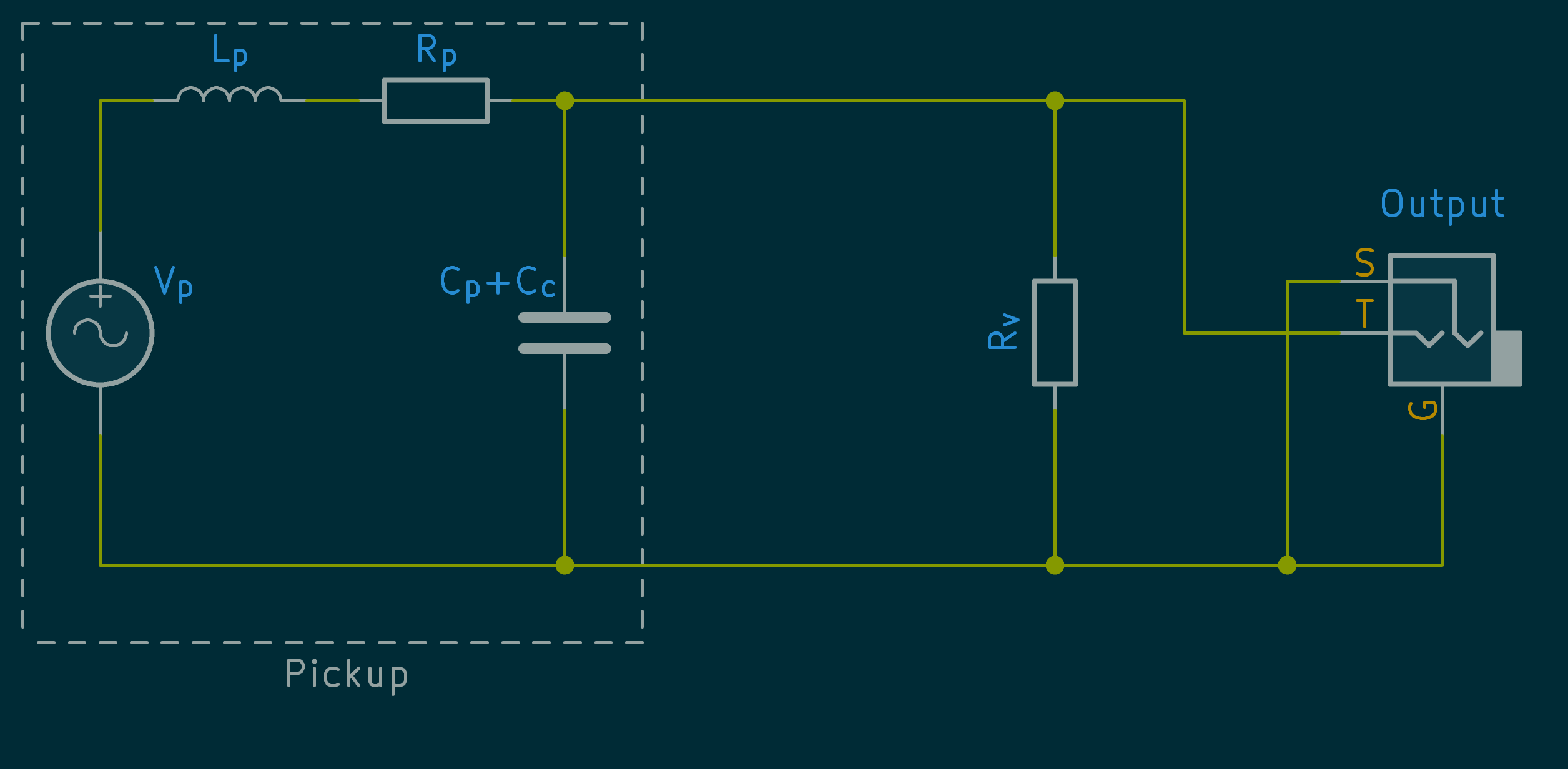
Here \(C_p + C_c = C_{p+c}\) is the combined capacitance of the pickup and cable. When the volume control is set to maximum these are effectively in parallel and can therefore be summed. \(C_p\) can be measured separately (and rather more easily as an open circuit guitar cable is accurately modelled as a single capacitor for audio frequencies) and then subtracted out to get the capacitance of just the pickup if required.
The rest of this article will cover measurements to find the values for these components and then provide some typical values based on my measurements.
Measurement Setup~
Measuring the impedance of a guitar is trivially easy with an Analog Discovery as this can be configured as a vector network analyser.
Actual VNAs (for example the various versions of the NanoVNA) can be bought for similar or less money but do not typically cover the full audio band if they cover it at all as they are targeted at RF use.
Equivalent measurements can be taken with a signal generator and a two-channel oscilloscope but depending on which maths functions and measurement options the oscilloscope has this can be significantly more labour intensive.
An impedance analyser add-on can be bought separately for the Analog Discovery. Since I would prefer to measure a guitar by simply plugging it into the measurement device using a standard guitar cable I made my own simple adaptor with a ¼" jack.
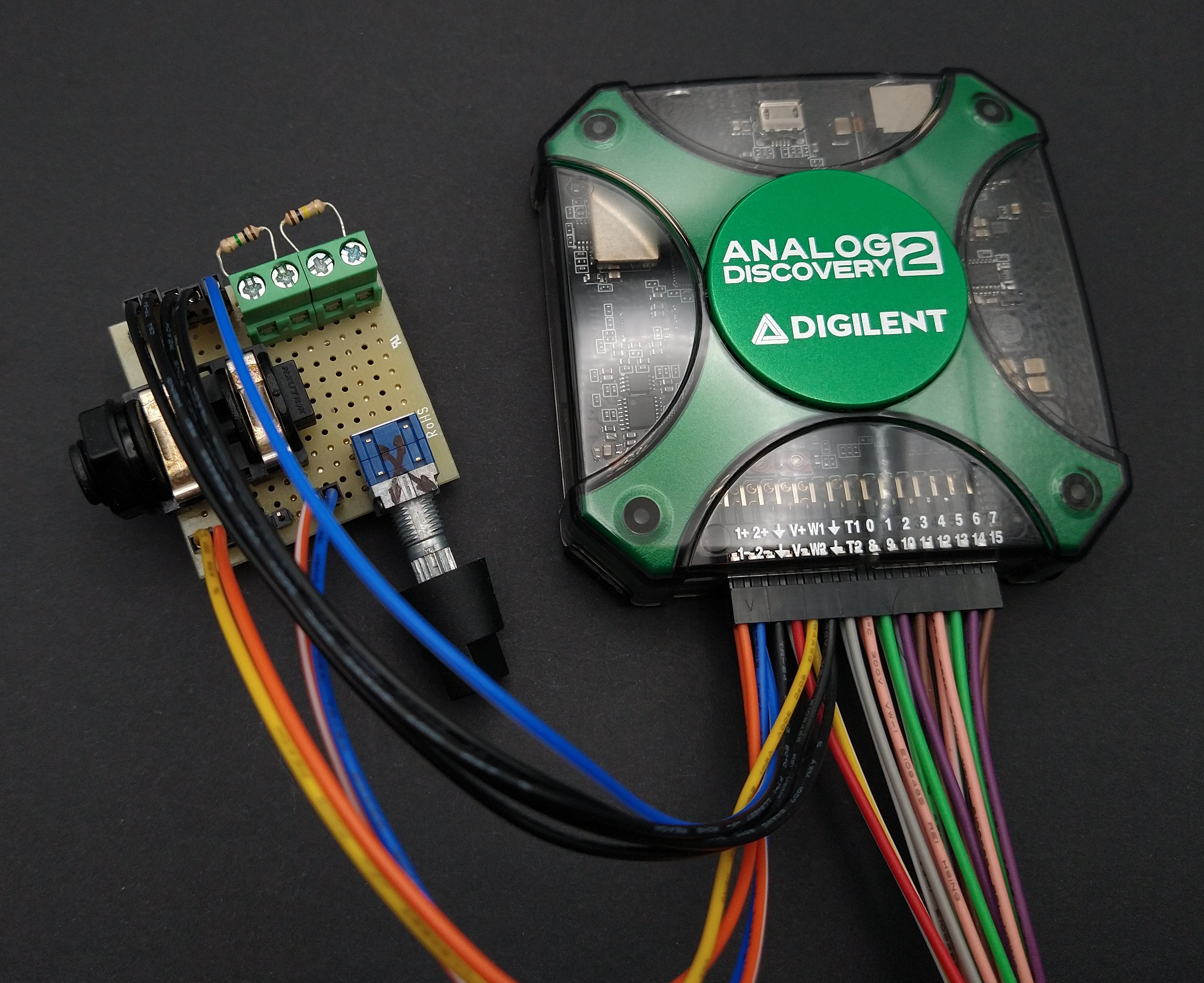
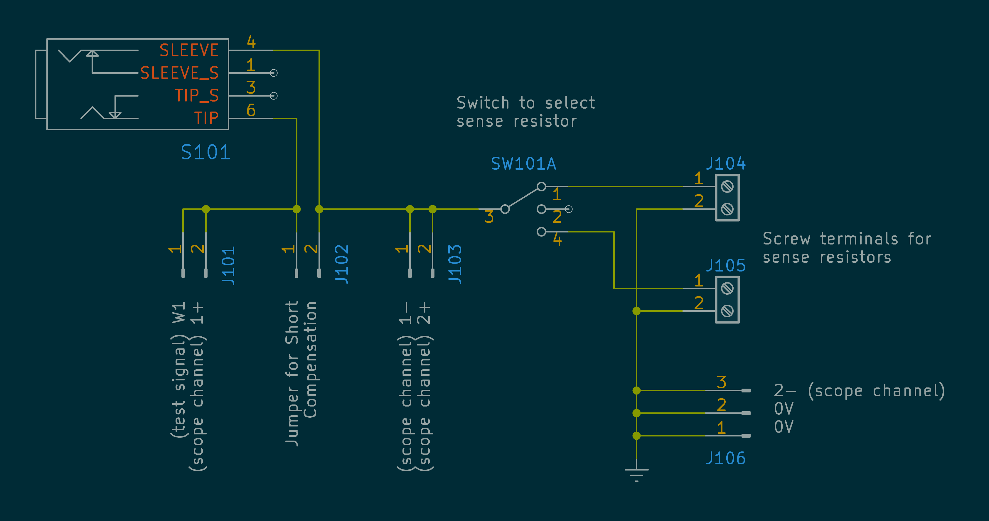
With this the Analog Discovery can supply a test signal into the guitar and then measure the voltage across both the guitar and the current-sensing resistor. The PC software for the Analog Discovery can convert these measurements into the impedance of the guitar.
Raw Data~
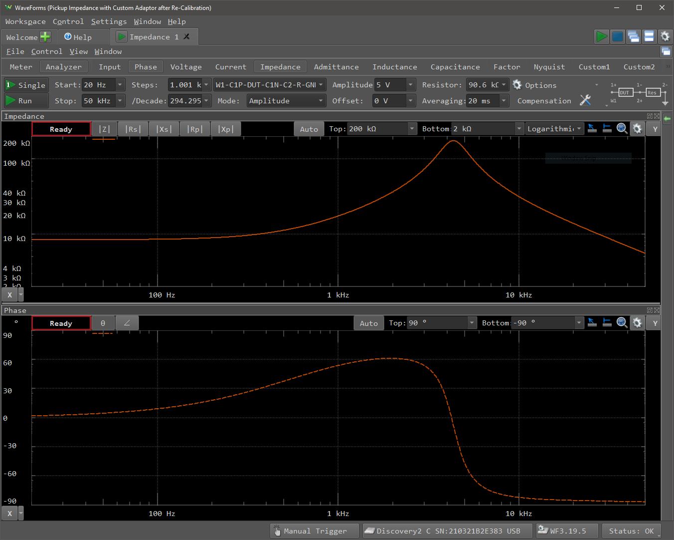
As can be seen from this screenshot the measurements are reassuringly close to a typical frequency response for a under-damped second-order system. The pickup equivalent circuit is very close to an RLC series network so this is the expected frequency response. It can also be seen that the measurements include both the phase and amplitude of the impedance.
Analysis / Component Value Inference~
For the guitar that I am initially measuring (and most Stratocasters) the volume control resistance \(R_v = 250 \ \mathrm{k}\Omega\) at least nominally. It would be preferable to measure this value accurately but I cannot think of a way to do that without dismantling the guitar to get direct access to the potentiometer
Method 1 - Mostly Hand Calculations~
This is probably the simplest and easiest option. In fact, this approach is simple enough that most of the results can be obtained with simple multimeter or LCR meter readings if the measurement frequencies are known.
Pickup Resistance~
In the plot of the magnitude and phase of the guitar impedance above the phase is very nearly 0 ° at 20 Hz, which means that the impedance is effectively real at this frequency. There are two purely real element in the equivalent circuit so it can be inferred that
Or in other words at (or close to) DC the inductance of the pickup and the capacitance of the pickup and cable are both negligible. Hence, this value could also be found from a standard DC resistance measurement. If a frequency sweep of the impedance is not being used you just have to be confident that the resistance measurement is being made at a frequency for which the impedances of the pickup inductance and capacitance are negligible.
Pickup (+Cable) Capacitance~
Similarly the phase from 20 to 50 kHz is very nearly -90 ° so in this region the resistance and inductance of the pickup must be negligible. Hence, rearranging the formula for the impedance of a capacitor allow calculation of the capacitance.
This could also be measured with a multimeter or RLC meter as long as the measurement frequency is safely above the resonant peak in the impedance frequency response. For most pickups it is probably safe to say that a capacitance measurement above 20 kHz will give a fairly accurate measurement.
Pickup Inductance~
Hand-calculable~
From the graph of the impedance it is reasonable to assume that damping of the network is relatively low as the peak is more than ten times the low frequency value. If one neglects the effect of damping on the natural frequency a reasonable approximation of the inductance can be found by re-arranging the equation for the undamped resonant frequency of a series RLC circuit [\(\ref{eq3}\)] as this only depends on the inductance and the capacitance and we have already estimated the capacitance.
The resonant frequency \(\omega_0\) can be read from the plot above. In this case the peak is at \(4.33 \ \mathrm{kHz}\) and so \(\omega_0 = 27.3\times10^3 \ \mathrm{rad/s}\).
Slightly more Accurate, Numerical Solution~
This undamped natural frequency is not the exact frequency at which the impedance is greatest when there is damping involved. When considering the amplitude response of an RLC circuit there are similar concepts of "undamped" and "damped" natural frequency. This Wikipedia page covers most of the maths for the amplitude responses i.e. the voltage and current through the network vs frequency.
The expression for the actual peak frequency \(\omega_d\) is little messy to derive. It can be expressed relatively neatly using the standard parameters that are used to characterise RLC networks. Namely the undamped natural frequency \(\omega_0 = \frac{1}{\sqrt{L_p C_{p+c}}}\) as used above, the attenuation \(\alpha = \frac{R_p}{2 L_p}\) and the damping factor \(\zeta = \frac{\alpha}{\omega_0} = \frac{R_p}{2} \sqrt{\frac{C_p}{L_p}}\).
In terms of just the component values this expression is
This can technically be solved symbolically for \(L_p\) but the result is ridiculously unwieldly as it ends up being a quartic equation in \(L_p\). Numerically solving the equation using the values for the other component values found above yields
In this case this value is close (within 4%) to the value found by the simpler method of \(\ref{eq3}\) and \(\ref{eq4}\). This is because the extra factor in \(\ref{eq5}\) that relates \(\omega_d\) to \(\omega_0\) is very close to unity for small values of \(\zeta\) i.e. for pickups that have a relatively sharp resonance in the impedance vs frequency plot and when \(R_p \ll R_v\). For pickups with a much wider resonant peak this factor may be significant. If the damping is high enough there may not be a discernible peak, or it may at least be very hard to determine the frequency of the peak accurately.
Method 2 - Entirely Numerical~
Since the impedance of the network only contains three unknown variables (or four if the volume control resistance is treated as an unknown) and is of a known form it should be relatively easy to use curve-fitting techniques to find a "least-squares" set of component values.
This method should also work where Method 1 fails, for example if the impedance at low frequencies is not effectively resistive or if there is no clear resonant peak.
I have tested this using the scipy.optimize.curve_fit function, an example Python script is shown below. The PC software for the Analog Discovery is called Waveforms and can export the measurements as CSV files. The script loads that file and then tries to find component values to get the closest possible to the measured \(|Z|\) data.
To do this it needs a Python function that represents the expression for the magnitude of the impedance. This expression is
which is implemented in fit_func below.
import pandas as pd
import numpy as np
from scipy.optimize import curve_fit

# Analog Discovery Software outputs a pre-amble with extra information about the
# configuration that was used. These lines all start with '#' so use the
# comment argument to skip them.
data = pd.read_csv(data_path, comment="#", index_col=0)

# Assign the frequency values to a variable with a shorter name and construct
# the magnitude of the impedance from the real and imaginary parts.
freqs = data.index.values
data["|Z|"] = np.abs(data["Real (Ohm)"] + 1j*data["Imag (Ohm)"])


def fit_func(f, R, R_v, C, L):
    """Expression for |Z|."""
    omega = 2.0*np.pi*f
    return np.sqrt(R_v**2*((L*omega)**2 + R**2) /
        ((C*L*R_v*omega**2)**2 + (C*R*R_v*omega)**2 -2*C*L*R_v**2*omega**2 +
        (L*omega)**2 + R**2 + 2.0*R*R_v + R_v**2))


initial_parameter_guess = (5.0e3, 200.0e3, 100.0e-12, 1.0)

popt, _ = curve_fit(fit_func, freqs, data["|Z|"],
                    p0=initial_parameter_guess)

print(popt)
Running this with the data that I have been using for the calculations above yields the following values. Note that I set it up to find an optimal value of \(R_v\) rather than using the nominal value as I found that this allowed it to find a better fit.
I found that providing scipy.optimize.curve_fit with reasonable initial guesses for the parameter values helped find a good fit. I experimented with using the bounds parameter to restrict the valid range of values for each parameter but I found that this actually made the fits much worse.
The table below shows the values found by the curve fit and compares the values found by the previous more manual method.
| Component | Values from Curve Fit | Values from Manual Methods | Difference between Estimates |
|---|---|---|---|
| \(R_p\) | 8.68 kΩ | 8.61 kΩ | 0.81 % |
| \(R_v\) | 291 kΩ | 250 kΩ (nom.) | 16 % |
| \(C_{p+c}\) | 613 pF | 579 pF | 5.9 % |
| \(L_p\) | 2.24 H | 2.41 H | 7.6 % |
The differences in these values are relatively small. If the volume potentiometer value were measured directly they probably would be even smaller. As it stands either method is probably adequately accurate for most general purpose simulations as there is likely to be variation between nominally identical guitars that is of comparable magnitude.
Comparison of Results~
The image below shows the measured impedance (magnitude) and the calculated impedance using \(\ref{eq9}\) and each of the sets of component values. The differences betwen the lines are not terribly visible so the bottom plot is the percentage difference between each kind of estimate and the measured data.
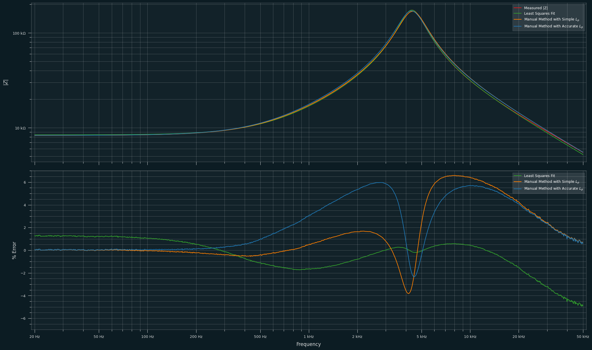
The "manual method" with the simpler calculation for \(L_p\) has a maximum error of 6.5%. The more accurate method for estimating \(L_p\) reduces the maximum error to 6%. The least-squares curve-fit method has maximum (absolute) error of 4%.
The overall performance is broadly equivalent but it is worth noting that the curve-fit method does seem to estimate the behaviour around the peak in the impedance more accurately than the manual method. The manual method effectively achieves a minimum error at the lowest and highest frequencies in the measured data simply due to using the impedance values at those frequencies in the calculations.
Separating out Cable Capacitance~
For all the measurements above I was connecting the guitar to the Analog Discovery adaptor using an unbranded 3 m guitar lead. Measuring the capacitance of this cable i.e. between tip and ring with an LCR45 meter yielded \(C_c = 380 \ \mathrm{pF}\). This is 127 pF/m which is relatively high for a guitar lead but not outlandish.
This can be subtracted from the \(C_{p+c}\) values above to isolate the capacitance of just the guitar, which is the pickup capacitance plus any other sources of capacitance from the controls or internal wiring.
For my measurements \(C_p = 233 \ \mathrm{pF}\) for the curve fit method and \(C_p = 199 \ \mathrm{pF}\) for the more manual method.
Conclusion~
The image below summarises the values that were found by the slightly more accurate curve-fitting method.
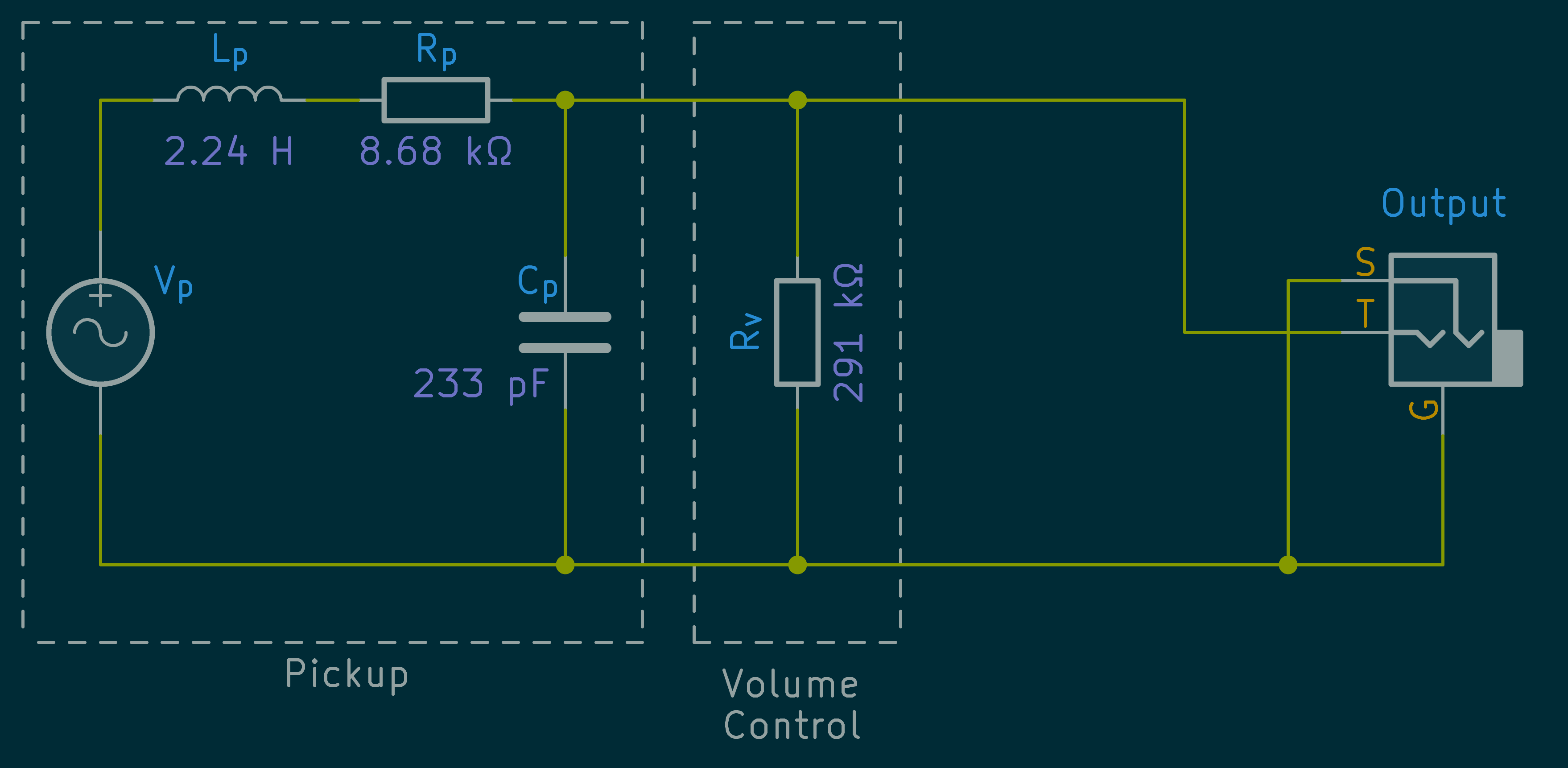
These values produce an equivalent circuit that matches the measured data to within a maximum absolute error of 4%.